AI for Survival Models

Real-World Clinical Data Overview

For our survival modeling analyses, we utilize publicly available clinical data from the TCGA-BRCA Pan-Cancer Atlas (2018). The file name is (brca_tcga_pan_can_atlas_2018_clinical_data.tsv). This dataset, widely used in cancer research, includes comprehensive clinical annotations for breast cancer patients.

In the dataset, there are 1,085 patients, of whom 145 experienced the event of interest (Progression) and 940 were censored (i.e., did not experience progression during the observation period). Our platform focuses on a subset of clinically and genomically relevant variables to enhance both the interpretability and predictive performance of survival models. By concentrating on these features, we reduce noise and ensure that the model outputs are meaningful for clinical decision-making. The variables considered include: Diagnosis Age: Age at diagnosis (continuous). Aneuploidy Score: Measurement of chromosomal instability. Buffa Hypoxia Score: Quantifies tumor hypoxia levels. Time Since Initial Pathologic Diagnosis: Duration since diagnosis (continuous). Fraction Genome Altered: Proportion of the genome with alterations. MSI Mantis Score: Microsatellite instability measured via the MANTIS tool. MSIsensor Score: Microsatellite instability measured via the MSIsensor tool. Mutation Count: Total number of mutations detected in the tumor. Progression-Free Survival (months): Time the patient remains progression-free. Ragnum Hypoxia Score: Additional hypoxia-related metric. Sex: Categorical variable. Tumor Break Load: Measure of genomic breaks in tumor DNA. TMB (Nonsynonymous): Tumor mutation burden considering nonsynonymous mutations. Winter Hypoxia Score: Additional hypoxia metric to capture tumor oxygenation levels. By focusing on these clinically and genomically informative features, the platform balances model complexity with interpretability, enabling robust and actionable predictions of patient-specific outcomes.

Interpretation of the Cox Proportional Hazards Model Output

Variables (Covariates) in the Model

The model includes these covariates representing clinical or biological measurements, estimated simultaneously for their effect on survival (hazard):

Diagnosis Age: Age at diagnosis (continuous).
Aneuploidy Score: Chromosomal instability measurement.
Buffa Hypoxia Score: Quantifies tumor hypoxia.
Last Communication Contact from Initial Pathologic Diagnosis Date: Time elapsed since diagnosis (continuous).
Fraction Genome Altered: Proportion of genome altered.
MSI Mantis Score: Microsatellite instability (mantis tool).
MSIsensor Score: Microsatellite instability (msisensor tool).
Mutation Count: Number of mutations detected.
Progress Free Survival (months): Time without progression.
Ragnum Hypoxia Score: Additional hypoxia score.
Sex: Categorical variable.
Tumor Break Load: Genomic breaks measure.
TMB (Nonsynonymous): Tumor mutation burden.
Winter Hypoxia Score: Another hypoxia score.

Coefficients (β) and Hazard Ratios (HR)

The model estimates log hazard ratios (β) and corresponding hazard ratios (HR = exp(β)) indicating how a 1-unit increase affects risk:

HR > 1: Increased hazard (worse survival).
HR < 1: Decreased hazard (better survival).

Variable	Coef (β)	HR (exp(β))	95% CI HR Lower	95% CI HR Upper	p-value	Interpretation
Buffa Hypoxia Score	-0.0443	0.957	0.922	0.993	0.0186	Each unit ↑ decreases hazard by 4.3% (protective)
Last Communication Contact Time	-0.0039	0.996	0.995	0.997	2.2e-19	Longer time since diagnosis strongly lowers hazard
Fraction Genome Altered	-3.3045	0.037	0.0043	0.316	0.0026	High fraction altered strongly protective
Progress Free Survival (months)	-0.0606	0.941	0.925	0.957	4.1e-12	Longer PFS time decreases hazard
Ragnum Hypoxia Score	0.0418	1.043	1.005	1.082	0.0249	Higher score raises hazard by ~4.3%
Winter Hypoxia Score	0.0466	1.048	1.015	1.081	0.0037	Higher score raises hazard by ~4.8%

Non-significant covariates (p > 0.05): Diagnosis age, aneuploidy score, MSI mantis score, MSIsensor score, mutation count, sex, tumor break load, TMB (nonsynonymous).

P-values and Statistical Significance

P-values test the null hypothesis β = 0 (no effect). Variables with p < 0.05 are statistically significant. Your model contains highly significant predictors (e.g., last communication contact p < 1e-18), and some borderline (diagnosis age p=0.066) or non-significant variables (sex p=0.44).

Confidence Intervals (95%)

Confidence intervals (CI) provide plausible effect ranges. Significant variables have CIs for HR that do not cross 1, reinforcing the effect. For example, Buffa hypoxia score HR CI: 0.922 – 0.993 (protective). Non-significant covariates often have CIs including 1.

Model Fit and Diagnostics

Log-Likelihood Ratio Test: 224.59 with 14 degrees of freedom, p ≈ 5e-40, indicating strong model fit over null.
Concordance Index (c-index): 0.942, indicating excellent prediction accuracy (1 = perfect, 0.5 = random).
Residuals: Mean deviance residual ~ -0.12 (near zero suggests good fit). Other residuals like Schoenfeld or Martingale not reported but recommended for diagnostics.
Proportional Hazards Assumption: Not formally tested here; Schoenfeld residuals recommended.
Linearity of Continuous Covariates: Not assessed; Martingale residual plots advised.

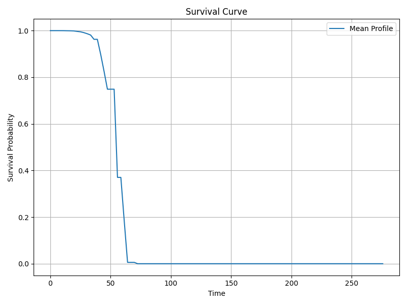
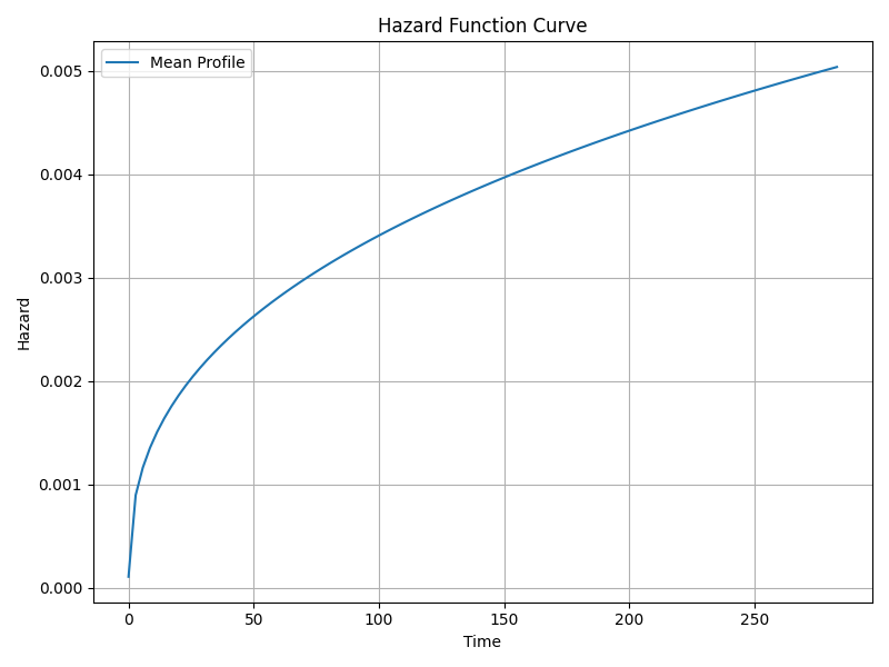
Survival and Hazard Functions

The Cox model is semi-parametric and estimates hazard multiplicatively relative to baseline hazard. Although not directly reported, key functions include:

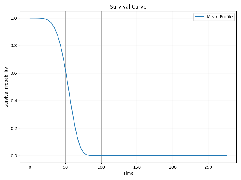
Survival function s(t): Probability of surviving beyond time t.
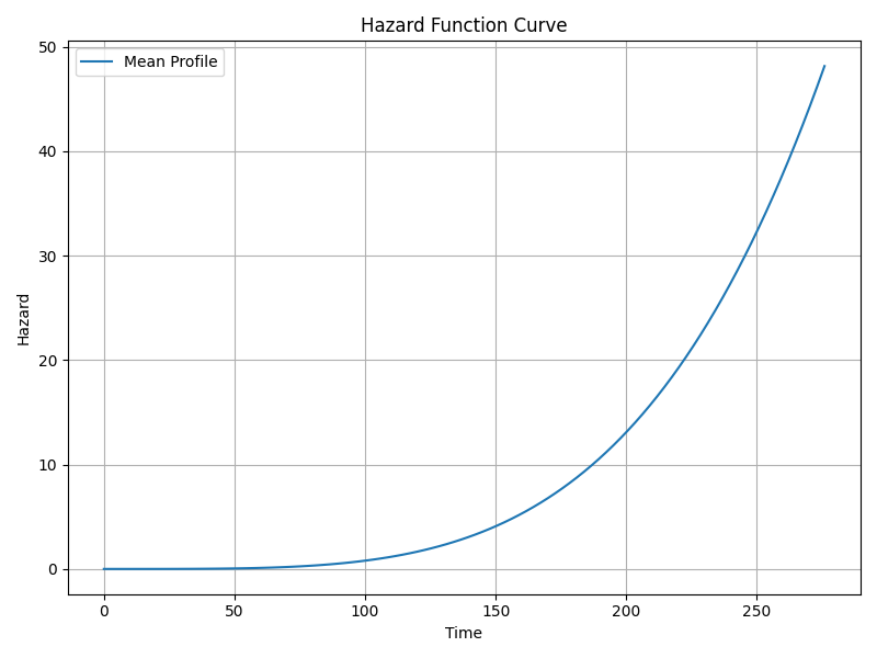
Hazard function h(t): Instantaneous risk of event at time t.
Cumulative hazard function H(t): Integrated hazard over time.

The baseline survival curve is available and visualized below.

Visualizations

Suggested Diagnostic Checks

To validate model assumptions and improve reliability, consider:

Proportional Hazards Assumption: Use Schoenfeld residuals plots and tests to check if hazard ratios remain constant over time.
Linearity of Continuous Covariates: Martingale residual plots can assess if covariates relate linearly to log hazard; consider transformations if needed.
Influential Observations and Outliers: Identify via deviance residuals and leverage diagnostics.
Goodness-of-fit: Use Cox-Snell residual plots to assess overall fit.

Using the Model for Prediction on New Data

You can predict survival probabilities or hazard for new patients by:

Calculate the linear predictor: LP = β₁x₁ + β₂x₂ + ... + βₖxₖ for the new covariate values.
Estimate relative hazard: HR = exp(LP).
Apply the baseline survival function S₀(t) (estimated from training data) scaled by the relative hazard to get predicted survival: S(t|x) = S₀(t)^{HR}.
Use available baseline hazard or survival curve (e.g., from survival_curve.png) or retrieve baseline hazard from the fitted model object in code.

In practice, software packages (e.g., lifelines, R's survival) provide functions for prediction, including confidence intervals.

Summary of Key Findings

The model is highly significant and predicts survival well (c-index 0.942).
Protective factors (lower hazard): buffa hypoxia score, last communication contact time, fraction genome altered, progress free survival.
Risk factors (higher hazard): ragnum hypoxia score, winter hypoxia score.
Some clinical variables like age and sex are not statistically significant in this model.
Hazard ratios quantify effect size, e.g., each unit increase in winter hypoxia score increases hazard by 4.8%.
Model assumptions (proportional hazards, linearity) require further testing.
Residual diagnostics and time-dependent effects were not assessed but are recommended for validation.

Log-Normal Survival Model Interpretation

Model Equation

The log-normal survival model assumes the log of survival time follows a normal distribution with mean μ and standard deviation σ. The location parameter μ is modeled as:

      μ = β₀ + β₁ × aneuploidy score + β₂ × buffa hypoxia score + ... + β₁₄ × winter hypoxia score
    

The scale parameter is modeled separately by the log of σ:

      log(σ) = γ₀
    

Covariates Explanation

Aneuploidy score: Chromosomal instability measure in tumor cells.
Buffa hypoxia score: Gene expression signature indicating tumor hypoxia.
Diagnosis age: Patient age at diagnosis.
Fraction genome altered: Proportion of genome with copy number changes.
Last communication contact: Time from diagnosis to last patient contact (days).
MSI mantis score: Microsatellite instability score from mantis tool.
MSIsensor score: Microsatellite instability score from msisensor tool.
Mutation count: Number of mutations detected.
Progress free survival (months): Time without disease progression.
Ragnum hypoxia score: Another hypoxia-related score.
Sex: Patient sex (binary).
TMB (nonsynonymous): Tumor mutation burden (nonsynonymous mutations).
Tumor break load: Measure of chromosomal breakpoints/rearrangements.
Winter hypoxia score: Additional hypoxia-related score.
Intercept (mu_): Baseline log survival time.
Intercept (sigma_): Baseline log scale parameter.

Coefficients Interpretation

Each coefficient βᵢ represents the effect of one unit increase in the covariate on the log of survival time. A positive coefficient indicates longer expected survival time; a negative coefficient indicates shorter survival.

Hazard Ratios (Exponentiated Coefficients)

Exponentiated coefficients exp(β) are interpreted as multiplicative effects on survival time (not hazards). Values > 1 indicate longer survival time; < 1 indicate shorter.

Example: Diagnosis age has exp(β) = 0.9934, meaning each additional year decreases expected survival to ~99.34% of the previous.

Statistical Significance (p-values)

Significant predictors (p < 0.05) include:

Diagnosis age: p = 0.0188
Last communication contact: p = 0.00319
MSI mantis score: p = 0.047
Progress free survival (months): p = 8.7e-16
Intercepts (mu_ and sigma_): highly significant

All other covariates are not statistically significant predictors of survival time.

Confidence Intervals (95%)

For significant variables, 95% CIs for coefficients exclude zero and for exp(β) exclude one, confirming significance.

Diagnosis age: coef CI: [-0.0121, -0.0011], exp(coef) CI: [0.9879, 0.9989]
Last communication contact: tight positive CI for coef and exp(coef) > 1
MSI mantis: exp(coef) CI ~ [0.0147, 0.97], indicating protective effect

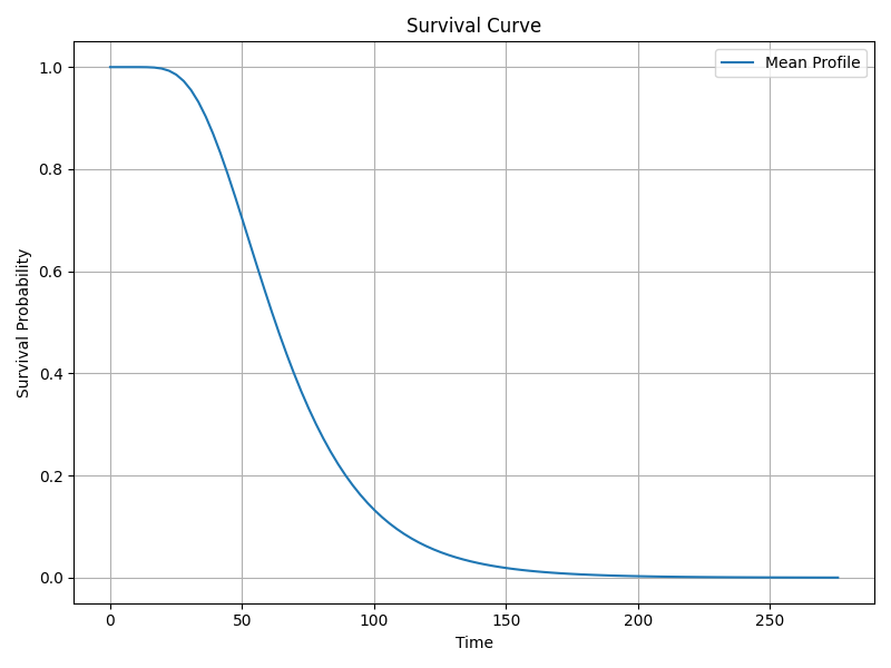
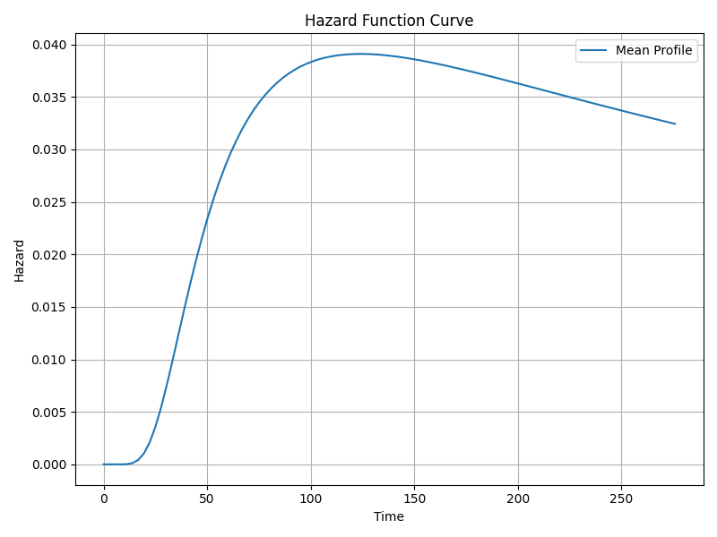
Survival, Hazard & Cumulative Hazard Functions

The survival function s(t) gives probability of surviving beyond time t, computed from the normal distribution of log(t) with mean μ and scale σ.

The hazard function h(t) represents instantaneous risk at time t. For log-normal, hazard is non-monotonic, rising then falling.

The cumulative hazard function is the integral of the hazard over time (not shown explicitly).

Shape and Scale Parameters

The scale parameter σ controls spread of log survival times and is modeled by the intercept under 'sigma_'.

Scale coefficient: -0.8644
Exponentiated scale coefficient: 0.4213
Highly significant (p ≈ 7.7e-21)

Log-normal models do not have a separate shape parameter like Weibull models.

Model Fit and Statistics

Log-likelihood ratio test statistic: 159.36
p-value: 9.53e-27 (highly significant)
Degrees of freedom: 14
AIC: 670.92
BIC: 651.94

These indicate the model fits significantly better than a null model, but fit should be compared to alternative models.

Model Diagnostics

No residuals (deviance, Cox-Snell, Martingale, Schoenfeld) or proportional hazards tests are reported.

Proportional hazards assumption is not relevant for this parametric log-normal model.

No diagnostics for linearity or time-dependent effects were performed.

Concordance Index (C-Index)

The model's c-index is 0.040, which is very low compared to random chance (~0.5). This suggests poor predictive discrimination on the test data.

Median and Mean Survival Times

Mean survival time: 68.44 units (likely months)
Median survival time: 62.63 units

Summary of Key Significant Effects

Variable	Coefficient (β)	exp(β)	p-value	Interpretation
Diagnosis age	-0.0066	0.9934	0.0188	Each additional year reduces expected survival time by ~0.66%.
Last communication contact	0.000138	1.00014	0.00319	Longer follow-up associated with slightly longer survival.
MSI mantis score	-2.123	0.120	0.047	Higher score strongly associated with longer survival.
Progress free survival (months)	0.0158	1.0159	8.7e-16	Longer progression-free survival strongly predicts longer overall survival.
Intercept (mu_)	4.289	72.92	~0	Baseline log survival time.
Intercept (sigma_)	-0.864	0.421	~0	Scale parameter (log survival time variability).

Recommendations for Diagnostics & Prediction

Model diagnostics: Perform residual analyses (Cox-Snell, Martingale), check linearity of continuous covariates and consider time-dependent effects if data allows.
Predictive performance: Explore alternative parametric models (Weibull, Gompertz) or flexible methods (Cox PH, random survival forests) since current c-index is poor.
Proportional hazards assumption: Not relevant for log-normal, but check if Cox model is considered.
Prediction for new data: Use estimated coefficients to compute μ for new covariate values, then derive survival probabilities from the log-normal distribution:
```
μ_new = β₀ + Σ(βᵢ × xᵢ_new)
σ = exp(γ₀)
S(t) = 1 - Φ[(log(t) - μ_new) / σ]
        
```
where Φ is the standard normal CDF.

Weibull Survival Model Interpretation

1. Explanation of Variables (Covariates)

Aneuploidy score: continuous score of chromosomal abnormality.
Buffa hypoxia score: hypoxia-related gene signature score.
Diagnosis age: patient age at diagnosis.
Fraction genome altered: proportion of genome with copy number alterations.
Last communication contact: time since diagnosis to last follow-up contact.
MSI Mantis score: microsatellite instability score from Mantis tool.
MSIsensor score: alternative microsatellite instability score.
Mutation count: total detected mutations.
Progress free survival (months): time until progression or last follow-up.
Ragnum hypoxia score: another hypoxia signature.
Sex: categorical variable.
TMB (nonsynonymous): tumor mutational burden for nonsynonymous mutations.
Tumor break load: measure of chromosomal breakage.
Winter hypoxia score: additional hypoxia signature.
Intercepts: baseline hazard (lambda_) and shape parameter (rho_).

2. Coefficients (β) and Hazard Ratios (HR = exp(β))

Coefficients represent effects on the scale parameter (λ). Positive β → increased hazard (shorter survival), negative β → decreased hazard (longer survival).

Covariate	β (Coef.)	HR = exp(β)	95% CI for HR	p-value	Interpretation
Diagnosis age	-0.0074	0.993	(0.988, 0.997)	0.00257	Older age significantly lowers hazard (longer survival).
Buffa hypoxia score	0.00637	1.006	(1.0001, 1.013)	0.045	Weak significant increase in hazard with higher hypoxia.
Last communication contact	0.000246	1.00025	-	≪ 0.001	Very significant hazard increase with follow-up time.
MSI Mantis score	-1.703	0.182	(0.034, 0.965)	0.045	High MSI Mantis score strongly reduces hazard.
Progress free survival (months)	(Not listed explicitly)	(Not listed)	-	≈ 4.7e-18	Strong positive association with hazard.
Ragnum hypoxia score	(Not listed explicitly)	(Not listed)	-	0.046	Weakly significant negative association (lower hazard).

Other covariates such as aneuploidy score, fraction genome altered, sex, mutation count, etc., were not statistically significant (p > 0.05).

3. Model Parameters and Fit Statistics

Shape parameter (ρ intercept): Estimate: 1.619 (exp = 5.05), SE = 0.0935, p ≈ 3.86 × 10⁻⁶⁷
Interpretation: Since ρ > 1, hazard increases over time.
Scale parameter (λ intercept): Estimate: 4.103 (exp = 60.53), highly significant.
Controls timing/spread of survival distribution.
Log-Likelihood Ratio Test: Statistic: 176.48 (df=14), p ≈ 3.35 × 10⁻³⁰
Indicates model fits significantly better than null.
AIC: 650.58
BIC: 631.60
Concordance Index (C-index): Reported as 0.040 on test set.
Interpretation: Extremely low predictive accuracy, indicating poor discrimination.
Median & Mean Survival Time: Median: 53.89 units (likely months)
Mean: 53.23 units

4. Diagnostic Checks & Model Assumptions

Residuals: Not reported (no deviance or martingale residuals available).
Proportional hazards assumption: Not tested; requires Schoenfeld residuals or log-log plots.
Linearity of continuous covariates: Not assessed; would require martingale residual plots.
Time-dependent effects: Not included or tested.

5. Visualizations

6. Using the Model for Prediction on New Data

To predict survival probabilities or hazard for new patients:

Input patient covariate values corresponding to the model variables.
Calculate the linear predictor: LP = β₁x₁ + β₂x₂ + ... + βₙxₙ.
Obtain the scale parameter λ = exp(LP) for the Weibull distribution.
Use the shape parameter ρ (estimated intercept, ~1.619).
Compute survival function at time t:
S(t) = exp[-(λ * t)^ρ].
Compute hazard function:
h(t) = λ^ρ * ρ * t^(ρ-1).
Use these functions to estimate survival probabilities or hazard risk at desired time points.

Software packages like lifelines in Python or survival in R can automate these calculations.

Summary

The Weibull model fits significantly better than null and suggests increasing hazard over time (shape > 1).
Significant covariates: diagnosis age (protective), buffa hypoxia score (hazard increasing), MSI Mantis score (strongly protective), progress free survival and last communication contact (both hazard increasing), ragnum hypoxia score (weakly protective).
Many other variables are not statistically significant.
Model shows poor predictive accuracy on test data (C-index = 0.04), indicating low discrimination.
Residual and proportional hazards diagnostics are missing and recommended for further validation.
Visualizations of survival and hazard functions provide insights into risk over time.