AI for Survival Models

Below is a comprehensive explanation of your weibull survival model output. Clarifications are made on which aspects are directly supported by the model output and which are not provided.

1. Coefficients (β) – Effect of Covariates on Hazard (or Time to Event)

The model reports coefficients (β) for each covariate in the scale parameter (lambda_), which in Weibull models affects the timing of the event.
Age coefficient ≈ -0.0018, indicating a very small negative effect on the scale parameter.
BMI coefficient ≈ 0.022, positive effect.
Height and Weight have very small negative coefficients.
The intercept for lambda_ is large and positive (~5.63), setting the baseline scale.
The shape parameter (rho_) has an intercept coefficient of ~0.80.

Interpretation: coefficients indicate the direction and magnitude of covariate effects on the scale parameter, relating to survival time in Weibull models. Smaller or negative coefficients imply longer expected survival (lower hazard), larger or positive coefficients imply shorter survival (higher hazard).

2. Hazard Ratios (HR) – Exponentiated Coefficients (HR = e^β)

HRs are provided as exp(coef) for each covariate under lambda_.
Age: HR = 0.998, very close to 1, indicating virtually no effect on hazard.
BMI: HR = 1.022, suggesting a 2.2% increase in hazard per unit increase in BMI (not statistically significant).
Height and Weight: HRs near 1 (0.9998 and 0.997 respectively), negligible effects.
Intercept HR is very large (~278), relating to baseline scale but limited direct interpretation for covariates.

Interpretation: no covariates show strong evidence of increasing or decreasing hazard substantially, as HRs are close to 1.

3. P-values – Statistical Significance of Covariate Effects

All covariates have non-significant p-values:
- Age: p = 0.684
- BMI: p = 0.181
- Height: p = 0.976
- Weight: p = 0.523
Intercepts for lambda_ and rho_ are highly significant (p < 0.001).
Likelihood ratio test p-value = 0.75, indicating the model with covariates is not significantly better than null.

Interpretation: no statistically significant evidence that any covariates affect survival time in this model.

4. Confidence Intervals (95%) – For Coefficients and Hazard Ratios

95% CIs for HRs include 1 for all covariates:
- Age HR CI: ~0.989 to 1.007
- BMI HR CI: ~0.99 to 1.06
- Height and Weight: similarly wide, including 1

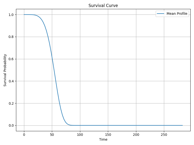
This confirms the lack of significant effect; intervals cross the null value of 1.

5. Survival Function S(t) – Probability of Surviving Beyond Time t

The survival function curve is visualized below. Numerical values are not reported here.

Survival Function Curve

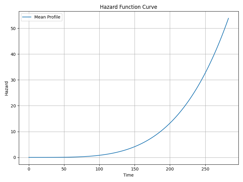
6. Hazard Function h(t) – Instantaneous Risk of Event at Time t

The hazard function curve is visualized below, showing the hazard change over time per the Weibull model.

Hazard Function Curve

7. Cumulative Hazard Function h(t)

No direct output or plot for cumulative hazard is provided. It can usually be derived from the hazard or survival functions.

8. Shape Parameter – Governs Hazard Behavior Over Time

Shape parameter rho_ coefficient = 0.7976 (log scale), with exp(coef) = 2.22.
Interpretation in Weibull models:
- If ρ > 1, hazard increases over time.
- If ρ < 1, hazard decreases over time.
Here, ρ ≈ 2.22 > 1, so hazard is increasing with time.
Statistically highly significant (p ≈ 3×10^-13).

The hazard rate increases over time in this cohort.

9. Scale Parameter – Affects Timing/Spread of Survival Distribution

Related to lambda_, determined by intercept and covariates. The intercept is significant and large, setting baseline survival time scale. Covariates have small, non-significant effects on scale.

10. Log-Likelihood – Measure of Model Fit

Likelihood ratio test statistic = 1.93, p = 0.75.
No significant improvement over null model.
Explicit log-likelihood value not provided.

11. AIC / BIC – Model Selection Criteria

AIC = 725.22
BIC = 721.99
Lower values indicate better fit, but need comparison to alternatives.

12. Residuals – Diagnose Model Fit and Assumptions

No residuals (Cox-Snell, Martingale, Schoenfeld, Deviance) reported. Mean deviance residuals are "not available".

13. Concordance Index (C-index)

C-index = 0.538 on test data.
Values close to 0.5 indicate random prediction; 0.538 is only slightly better, suggesting poor predictive accuracy.

14. Proportional Hazards Assumption

Weibull is a parametric model with implicit PH assumption.
No PH tests (e.g., Schoenfeld residuals) reported here.

15. Linearity of Continuous Covariates

Not assessed or reported in this output.

16. Time-Dependent Effects

No time-dependent covariates or tests reported.

17. Median and Mean Survival Time

Mean survival time = 313.41 time units (days/months/years depending on data).
Median survival time = 300.02 time units.
Indicate central tendency of survival time for the cohort under model.

18. Restricted Mean Survival Time (RMST)

Not reported.

19. Cumulative Incidence Function (CIF)

Not applicable or reported; no competing risks model here.

20. Cause-Specific and Subdistribution Hazard Ratios

Not applicable or reported.

21. Posterior Distributions of Parameters

Not Bayesian; not reported.

22. Credible Intervals

Not Bayesian; only frequentist confidence intervals reported.

Summary

No covariates (age, bmi, height, weight) have statistically significant effects on survival time.
Hazard ratios are close to 1, with confidence intervals including 1.
Shape parameter indicates increasing hazard over time.
Model overall fit is weak: non-significant likelihood ratio test, low c-index (~0.54).
Mean and median survival times around 300 time units.
Survival and hazard function plots provided above for visual inspection.
No residual diagnostics, assumption tests, or advanced model diagnostics are reported.
Model may require reconsideration of covariate selection or functional form to improve predictive performance.

Suggested Diagnostic Checks

Residual analyses: Compute and inspect Cox-Snell, Martingale, Schoenfeld, and deviance residuals to assess model fit and PH assumption.
Proportional hazards assumption test: Although Weibull is parametric, verify PH assumption with residual-based tests or graphical checks.
Linearity checks: Use plots or spline terms to verify linearity of continuous covariates.
Influential observations: Identify outliers or influential data points using residuals or diagnostics.
Alternative models: Consider other parametric distributions or Cox PH models if fit is poor.

Using This Weibull Model for Prediction on New Data

To predict survival probabilities or hazard rates for new subjects:

Obtain the covariate values (age, bmi, height, weight) for the new data point.
Compute the linear predictor: LP = β₀ + β₁×age + β₂×bmi + β₃×height + β₄×weight.
Calculate the scale parameter λ from the linear predictor (e.g., λ = exp(LP) or as model specifies).
Use the shape parameter ρ (≈ 2.22) to define the Weibull distribution hazard function h(t) = ρ λ t^{ρ-1} and survival function S(t) = exp(-λ t^{ρ}).
Compute predicted survival probabilities at time points of interest using S(t).
Similarly, compute hazard or cumulative hazard as needed.

Note: Given the weak predictive power and non-significant covariates, predictions should be used cautiously and with awareness of the model limitations.

If you want help interpreting the graphs or require further model refinement, feel free to ask!